


No products in the cart.

Unlocking the Power of Trend Analysis
Want to predict future outcomes and make smarter decisions? Trend analysis methods are your key to understanding and capitalizing on emerging opportunities. This listicle provides practical insights into seven powerful trend analysis techniques. Learn how to identify hidden patterns and gain a competitive edge, regardless of your field. Whether you're a business leader or simply want to make more informed decisions, these methods will empower you.
This curated collection offers actionable advice and fresh perspectives. Each technique is presented with real-world examples and practical tips, ensuring you gain specific, applicable knowledge. Dive in to discover how these methods can help you:
- Anticipate market shifts: Stay ahead of the curve by identifying emerging trends.
- Make informed decisions: Base your choices on data-driven insights.
- Gain a competitive advantage: Understand trends to outperform competitors.
From simple techniques like moving averages to more complex methods such as ARIMA modeling, we'll cover a range of trend analysis approaches. You'll learn the pros and cons of each method, along with practical implementation tips. This listicle explores:
- Moving Averages
- Linear Regression Analysis
- Seasonal Decomposition
- ARIMA (AutoRegressive Integrated Moving Average)
- Exponential Smoothing
- Polynomial Trend Analysis
- Mann-Kendall Trend Test
Ready to uncover the secrets of trend analysis methods? Let's begin.
1. Moving Averages
Moving averages are a fundamental trend analysis method used to smooth out fluctuations in data and highlight underlying trends. They achieve this by calculating the average of data points over a specific period, effectively creating a trend line that reduces noise and reveals longer-term patterns. The "moving" aspect comes from continuously dropping the oldest data point in the set and adding the newest one as the analysis progresses. This continuous recalculation allows the average to adapt to new data and track changes in the trend.

How Moving Averages Work
The core concept behind moving averages is simple: averaging recent data points to filter out short-term volatility. For instance, a 5-day moving average takes the last five data points, calculates their average, and plots it on a chart. The next day, the oldest data point is dropped, the newest is added, and the average is recalculated.
This process repeats, creating a smoother line that represents the underlying trend, free from the daily spikes and dips. The period length (e.g., 5-day, 20-day, 50-day) determines the sensitivity of the moving average. Shorter periods react more quickly to recent changes, while longer periods provide a more stable, long-term view.
Applications of Moving Averages
Moving averages find applications across diverse fields. Here are some notable examples:
- Financial Markets: 50-day and 200-day moving averages are widely used in stock market analysis to identify trends and potential buy/sell signals.
- Sales Forecasting: Retail businesses employ moving averages, often 12-month averages, to forecast sales trends and manage inventory.
- Weather Analysis: Meteorologists use seasonal moving averages to track weather patterns and predict future conditions.
- Economic Indicators: Trend analysis of economic data like GDP often incorporates moving averages to identify long-term economic shifts.
Tips for Effective Use
To maximize the effectiveness of moving averages in your trend analysis, consider these practical tips:
- Multiple Time Periods: Use multiple moving averages with different periods (e.g., 10-day, 50-day, 200-day) together. This allows for a more nuanced understanding of both short-term and long-term trends. Confirmations across multiple timeframes strengthen the signal.
- Combine with Other Indicators: Moving averages are powerful on their own but even more effective when combined with other technical indicators. This helps validate trends and filter out false signals.
- Volatility Considerations: Adjust the period length based on the data's volatility. Highly volatile data benefits from longer periods to smooth out erratic fluctuations, while less volatile data can use shorter periods for more responsive trend tracking.
- Exponential Moving Averages (EMA): Consider using EMAs, a variation of the simple moving average, which gives greater weight to recent data. This makes EMAs more responsive to recent price changes and can be helpful in identifying emerging trends more quickly.
Why Moving Averages Matter
Moving averages are a crucial tool in trend analysis due to their ability to filter noise and reveal underlying patterns. They provide a simple yet effective way to understand the direction and strength of a trend. This clarity enables informed decision-making in various fields, from investment strategies to business planning. Their versatility and ease of implementation make them an essential method for anyone seeking to analyze and interpret data trends.
2. Linear Regression Analysis
Linear regression analysis is a powerful statistical method used to model the relationship between two variables by fitting a linear equation to observed data. One variable is considered the explanatory variable (independent variable), and the other is considered the dependent variable. The goal is to find the best-fitting straight line that minimizes the distance between the observed data points and the predicted values on the line. This line helps quantify the strength and direction of the trend, enabling predictions of future values based on the established relationship.
How Linear Regression Works
The core concept behind linear regression is finding the equation of a straight line that best represents the relationship between the two variables. This equation typically takes the form: y = mx + b, where 'y' is the dependent variable, 'x' is the independent variable, 'm' is the slope of the line (representing the change in 'y' for a unit change in 'x'), and 'b' is the y-intercept (the value of 'y' when 'x' is zero). The method aims to minimize the sum of the squared differences between the observed data points and the corresponding predicted values on the line. This minimization process results in the "line of best fit," which effectively captures the linear trend in the data.
Applications of Linear Regression
Linear regression finds wide application across various domains, including:
- Real Estate: Analyzing housing price trends over time based on factors like location, size, and amenities.
- Business Planning: Forecasting revenue growth by examining the relationship between marketing spend and sales figures.
- Climate Change: Analyzing temperature trends and predicting future climate patterns based on historical data.
- Demographics: Projecting population growth based on birth rates, mortality rates, and migration patterns.
Tips for Effective Use
To ensure accurate and meaningful results with linear regression, consider the following tips:
- Outlier Detection: Identify and handle outliers, as they can significantly skew the regression line and lead to inaccurate predictions. Outliers can be removed or adjusted based on domain expertise.
- Linearity Assumption: Validate the assumption that a linear relationship exists between the variables. If the relationship is non-linear, consider transformations or alternative models.
- R-squared Value: Use the R-squared value, a statistical measure, to assess the reliability of the trend. A higher R-squared value (closer to 1) indicates a better fit of the regression line to the data.
- Polynomial Regression: For non-linear patterns, explore polynomial regression, which uses higher-order terms to model curved relationships.
Why Linear Regression Matters
Linear regression is a valuable trend analysis method due to its ability to quantify the relationship between variables and provide predictive capabilities. Its ease of interpretation and wide applicability make it a fundamental tool for understanding and forecasting trends in various fields. By revealing the underlying linear patterns in data, linear regression empowers informed decision-making based on data-driven insights. The ability to predict future outcomes adds a significant dimension to trend analysis, facilitating proactive planning and effective resource allocation.
3. Seasonal Decomposition
Seasonal decomposition is a powerful trend analysis method that dissects time series data into its core components: trend, seasonality, and residual noise. This breakdown allows analysts to isolate and understand the underlying trend by separating predictable seasonal fluctuations from the overall directional movement. By removing the "seasonal noise," the true trend becomes more apparent, enabling better forecasting and strategic decision-making. This method is particularly useful when dealing with data that exhibits recurring patterns over time, such as sales figures, energy consumption, or weather data.
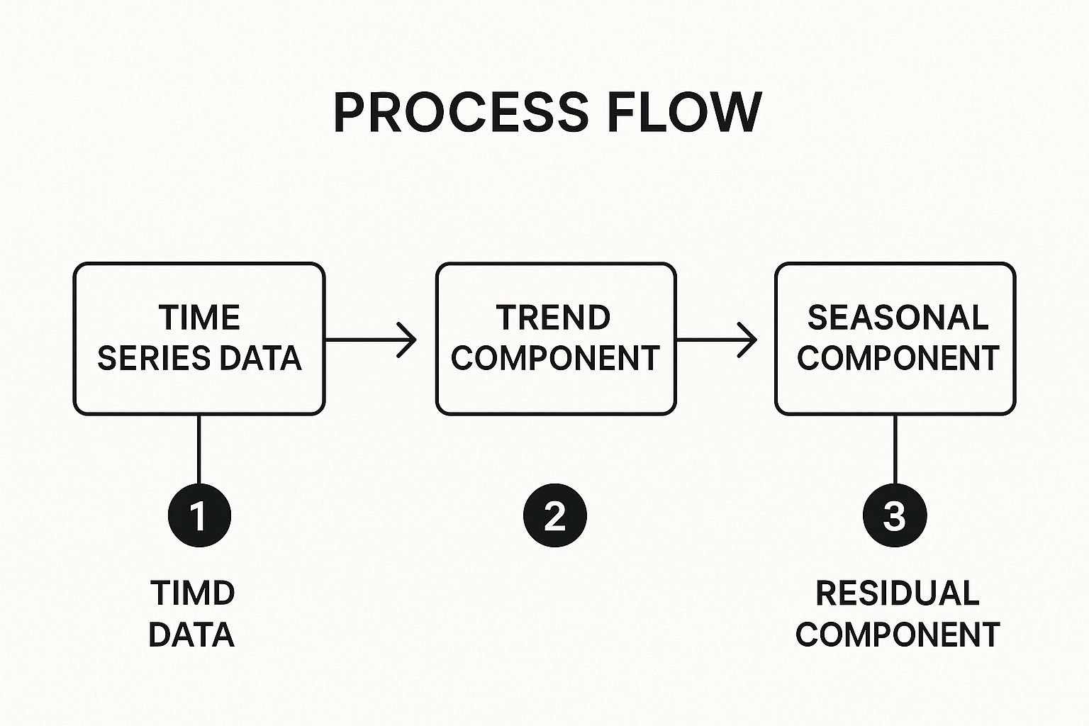
The infographic illustrates the process flow of seasonal decomposition, starting with the raw time series data and systematically extracting the trend, seasonal, and residual components. It highlights the step-by-step breakdown that allows for a clearer understanding of the underlying forces shaping the data.
The visualization clearly depicts how a time series is broken down into its fundamental parts: trend, seasonal component, and residual component, which allows for cleaner trend analysis and more informed business decisions.
How Seasonal Decomposition Works
The process typically involves several key steps:
- Data Collection: Gather historical time series data that spans multiple cycles of the seasonal pattern.
- Trend Identification: Determine the overall trend in the data using methods like moving averages or regression analysis.
- Seasonal Component Extraction: Isolate the repeating seasonal pattern. This involves calculating average deviations from the trend for each season.
- Residual Calculation: The remaining unexplained variation after removing the trend and seasonality is considered the residual or "noise" component.
Applications of Seasonal Decomposition
Seasonal decomposition has wide applications across various fields:
- Retail Sales: Analyze sales figures by removing holiday seasonality to understand underlying sales growth trends.
- Energy Consumption: Model energy usage patterns and forecast future demand based on seasonal variations and long-term trends.
- Tourism: Predict tourist arrivals by isolating seasonal fluctuations in travel patterns and identify underlying growth in tourism.
- Agriculture: Analyze commodity prices by accounting for seasonal crop cycles.
Tips for Effective Use
- Data Sufficiency: Utilize at least 2-3 years of data to reliably capture seasonal patterns. More data usually leads to more accurate decomposition.
- Evolving Seasonality: Consider that seasonal patterns can change over time. Regularly re-evaluate and update the seasonal component for accurate analysis.
- Business Sense Validation: Ensure that the extracted seasonal components make logical sense within the business context. This helps validate the decomposition results.
- Combined Analysis: Pair seasonal decomposition with other trend analysis methods, such as regression analysis, for a more comprehensive understanding of the data.
Why Seasonal Decomposition Matters
Seasonal decomposition is crucial for accurate trend analysis. It allows for informed decision-making by separating signal from noise. This separation helps to avoid misinterpreting short-term fluctuations as significant trend shifts. By understanding the true underlying trend, businesses and analysts can make more accurate forecasts, allocate resources effectively, and develop more robust long-term strategies.
4. ARIMA (AutoRegressive Integrated Moving Average)
ARIMA is a sophisticated statistical method used in trend analysis to model and forecast time series data. It combines autoregression (AR), differencing (I), and moving averages (MA) to capture complex temporal dependencies within the data. This makes ARIMA particularly effective for non-stationary data, which exhibits trends and changes in variance over time. Unlike simpler methods like basic moving averages, ARIMA can account for both the current value and past values, along with past forecast errors, when predicting future values.
How ARIMA Works
ARIMA models are defined by three parameters: (p, d, q). The "p" represents the order of the autoregressive component, indicating how many past values are used in the model. The "d" signifies the degree of differencing required to make the data stationary. Stationarity is a crucial assumption for ARIMA, meaning the data's statistical properties, like mean and variance, remain constant over time. Finally, "q" represents the order of the moving average component, specifying how many past forecast errors are incorporated.
The ARIMA model uses these parameters to create a mathematical equation that describes the relationships between the data points across time. This equation is then used to forecast future values. The process involves identifying the appropriate (p, d, q) values, estimating the model's coefficients, and validating its performance using statistical tests.
Applications of ARIMA
ARIMA models have a wide range of applications in various fields that require trend analysis and forecasting:
- Economic Forecasting: Central banks utilize ARIMA models to forecast macroeconomic indicators like inflation and GDP growth, informing monetary policy decisions.
- Demand Forecasting: Businesses use ARIMA to predict customer demand for products and services, optimizing inventory management and supply chain operations. Major retailers, for example, leverage ARIMA for supply chain demand planning.
- Financial Markets: Analysts apply ARIMA to model stock price movements and forecast market trends, aiding in investment decisions.
- Airline Passenger Demand Prediction: ARIMA can forecast passenger numbers, allowing airlines to optimize flight schedules and pricing.
Tips for Effective Use
Implementing ARIMA effectively requires careful consideration of several factors:
- Test for Stationarity: Before applying ARIMA, ensure your data is stationary. If not, use differencing to transform it. Common tests include the Augmented Dickey-Fuller (ADF) test.
- Model Selection (AIC/BIC): Use information criteria like AIC (Akaike Information Criterion) and BIC (Bayesian Information Criterion) to select the best ARIMA model. These criteria balance model fit with complexity.
- Residual Analysis: Validate the model by checking if the residuals (the differences between predicted and actual values) are white noise. This confirms that the model has captured most of the underlying pattern.
- Seasonal ARIMA (SARIMA): For data with seasonality, such as monthly sales figures, use SARIMA, an extension of ARIMA that accounts for seasonal patterns.
Why ARIMA Matters
ARIMA provides a powerful approach to trend analysis by modeling complex temporal dependencies. Its ability to handle non-stationary data and incorporate past information makes it suitable for a wide range of forecasting applications. While requiring a deeper understanding of statistical concepts than simpler methods, ARIMA offers a more robust and accurate way to understand and predict trends, leading to better informed decision-making across diverse fields.
5. Exponential Smoothing
Exponential smoothing is a sophisticated trend analysis method that forecasts future values by assigning exponentially decreasing weights to historical observations. This means recent data points hold greater influence than older ones, making it particularly effective for data exhibiting trends and seasonal patterns. Unlike simple moving averages, exponential smoothing doesn't treat all past data points equally, allowing for a more dynamic and responsive trend analysis. It excels in capturing evolving patterns and adapting to recent shifts in the data.
How Exponential Smoothing Works
Exponential smoothing uses a smoothing constant (alpha) between 0 and 1 to determine the weight given to each data point. A higher alpha gives more weight to recent data, making the forecast more reactive to recent changes. Conversely, a lower alpha emphasizes past data, leading to a smoother, less reactive forecast. The calculation involves recursively updating the forecast based on the previous forecast and the most recent actual data point, weighted by alpha.
This recursive nature allows the forecast to continuously adjust to new information, making it a valuable tool for trend analysis in dynamic environments. The choice of alpha is crucial and depends on the data's characteristics; more volatile data typically warrants a higher alpha.
Applications of Exponential Smoothing
The versatility of exponential smoothing makes it applicable across various domains:
- Inventory Management: Companies like Amazon and Walmart utilize exponential smoothing to forecast demand and optimize inventory levels. This helps minimize storage costs while ensuring product availability.
- Financial Forecasting: Banks and financial institutions employ exponential smoothing for predicting financial metrics, such as stock prices and interest rates. These forecasts inform investment decisions and risk management strategies.
- Production Planning: Manufacturing companies leverage exponential smoothing to forecast production needs and optimize resource allocation. This ensures efficient production schedules and minimizes waste.
- Website Traffic Prediction: Website administrators use exponential smoothing to predict traffic patterns and plan for capacity needs. This allows for proactive scaling of server resources and ensures optimal website performance during peak traffic periods.
Tips for Effective Use
To enhance the effectiveness of exponential smoothing in trend analysis, consider these practical tips:
- Smoothing Constant Selection: Carefully choose the smoothing constant (alpha) based on data volatility. Higher volatility requires higher alpha values for greater responsiveness to recent changes. Lower volatility allows for lower alpha values to capture long-term trends.
- Holt-Winters Method: For data with seasonal patterns, the Holt-Winters method, an extension of exponential smoothing, is particularly effective. This method incorporates seasonality into the forecast, improving accuracy for businesses with cyclical trends.
- Forecast Accuracy Monitoring: Continuously monitor the forecast accuracy and adjust parameters as needed. Data characteristics can change over time, requiring periodic adjustments to the smoothing constant or the chosen method.
- Judgmental Adjustments: Combine exponential smoothing forecasts with human judgment and domain expertise for strategic decisions. While statistical models provide valuable insights, human interpretation and context are essential for effective decision-making.
Why Exponential Smoothing Matters
Exponential smoothing stands out among trend analysis methods due to its ability to adapt to changing data patterns. By prioritizing recent observations, it provides more accurate and timely forecasts, particularly in volatile environments. Its flexibility, relative simplicity, and adaptability make it an invaluable tool for anyone seeking to understand and predict future trends. This allows for more informed and proactive decision-making in a variety of fields.
6. Polynomial Trend Analysis
Polynomial trend analysis is a sophisticated trend analysis method that goes beyond the limitations of linear models. It fits curved lines to data points, allowing it to capture non-linear trends that simpler methods like linear regression miss. These curves, represented by quadratic, cubic, or higher-order polynomials, provide a more nuanced understanding of trends exhibiting acceleration, deceleration, and cyclical patterns.
How Polynomial Trend Analysis Works
Unlike linear regression, which assumes a constant rate of change, polynomial trend analysis acknowledges that trends can change over time. A quadratic trend, for example, models data with a single curve, capturing accelerating or decelerating growth. Cubic and higher-order polynomials model more complex patterns with multiple inflection points, reflecting shifts in the trend's direction. The analysis involves finding the polynomial equation that best fits the historical data, enabling projections and insights into future behavior.
Applications of Polynomial Trend Analysis
The ability to model non-linear trends makes polynomial analysis applicable across diverse domains:
- Technology Adoption: The S-curve of technology adoption, where growth starts slowly, accelerates rapidly, and then plateaus, is effectively modeled using polynomial trends.
- Population Growth: Modeling population growth, especially when considering resource constraints, requires polynomial analysis to account for eventual slowing or decline.
- Product Lifecycle: The lifecycle of a product, from introduction to maturity and decline, often follows a non-linear path, making polynomial analysis suitable for market research and product planning.
- Economic Cycles: Economic growth cycles, marked by periods of expansion and contraction, lend themselves well to polynomial analysis for understanding and predicting economic fluctuations.
Tips for Effective Use
Successfully applying polynomial trend analysis requires careful consideration:
- Start Simple: Begin with low-order polynomials (quadratic or cubic) and only increase the order if the data warrants it. Higher-order polynomials can lead to overfitting, where the model fits the noise rather than the underlying trend.
- Cross-Validation: Employ cross-validation techniques to evaluate the model's performance on unseen data. This helps prevent overfitting and ensures the model generalizes well.
- Extrapolation Caution: Be cautious when extrapolating far beyond the existing data. Polynomial trends can diverge significantly outside the range of observed values, leading to unreliable predictions.
- Model Comparison: Compare multiple polynomial models using information criteria like AIC or BIC. These metrics help select the model that best balances fit and complexity.
Why Polynomial Trend Analysis Matters
Polynomial trend analysis provides a powerful tool for understanding complex trends that linear methods fail to capture. Its ability to model acceleration, deceleration, and cyclical patterns unlocks deeper insights into data behavior. This enhanced understanding allows for more accurate forecasting and more informed decision-making in fields ranging from technology forecasting to economic planning. While requiring more careful application than simpler methods, the potential for nuanced trend analysis makes polynomial trend analysis a valuable addition to any analyst's toolkit.
7. Mann-Kendall Trend Test
The Mann-Kendall trend test is a non-parametric statistical method used to identify monotonic trends in time series data. Unlike parametric tests, it doesn't assume a normal distribution, making it robust to outliers and suitable for various data types. This resilience is particularly valuable when analyzing environmental and climate data, which often exhibit non-normal distributions and contain outliers. The test determines whether a statistically significant increasing or decreasing trend exists within the data, without requiring the trend to be linear.
How the Mann-Kendall Test Works
The Mann-Kendall test assesses the direction of change between all possible pairs of data points in a time series. For each pair, it determines if the later value is greater than, less than, or equal to the earlier value. These comparisons are then summed to produce a statistic, S. A positive S suggests an upward trend, while a negative S indicates a downward trend. The statistical significance of S is then evaluated against a predetermined significance level (e.g., 0.05) to determine whether the observed trend is likely due to chance or represents a real trend.
Applications of the Mann-Kendall Test
The Mann-Kendall test finds broad applications in environmental and climate studies, among other fields:
- Climate Change Analysis: Organizations like NOAA and the EPA use the Mann-Kendall test to analyze long-term temperature and precipitation trends, providing crucial evidence for climate change studies.
- Water Quality Monitoring: The test helps assess trends in water pollutants, allowing researchers to monitor the effectiveness of water management strategies.
- Air Pollution Trend Detection: It is applied in urban areas to identify increasing or decreasing trends in air pollutant concentrations.
- Ecological Monitoring Programs: Long-term ecological monitoring projects utilize the Mann-Kendall test to detect changes in species populations or ecosystem health indicators.
Tips for Effective Use
For successful implementation of the Mann-Kendall test, consider these tips:
- Data Suitability: The test is ideal for environmental and ecological data where normality assumptions might not hold.
- Trend Magnitude: Combine the Mann-Kendall test with Sen's slope estimator to quantify the magnitude of the detected trend, providing a measure of change per time unit.
- Seasonal Data: For data exhibiting seasonality (e.g., monthly or quarterly data), apply the seasonal Mann-Kendall test to account for periodic fluctuations.
- Independence Assumption: Ensure the data points in your time series are independent. Autocorrelation can inflate the significance of the test and lead to erroneous conclusions.
Why the Mann-Kendall Test Matters
The Mann-Kendall test is a valuable trend analysis method due to its non-parametric nature and robustness to outliers. Its ability to detect monotonic trends in data with non-normal distributions makes it particularly relevant for environmental and climate science. The test provides statistically rigorous evidence for identifying and understanding long-term changes in various fields, contributing to informed decision-making in environmental management and policy. Its widespread use by prominent organizations like NOAA and the EPA underscores its importance in addressing critical global issues.
7 Methods Trend Analysis Comparison
| Method | Implementation Complexity 🔄 | Resource Requirements ⚡ | Expected Outcomes 📊 | Ideal Use Cases 💡 | Key Advantages ⭐ |
|---|---|---|---|---|---|
| Moving Averages | Low (simple formulas, easy to automate) | Low (basic computation) | Smooth trend lines, noise reduction | Financial markets, sales forecasting, economic analysis | Easy to implement, widely supported, reduces noise |
| Linear Regression Analysis | Medium (requires statistical methods) | Medium (data and software needed) | Quantitative trend direction, prediction with confidence | Business forecasting, scientific research, economic modeling | Provides statistical significance and predictions |
| Seasonal Decomposition | Medium-High (requires time series skills) | Medium (needs historical data) | Separates trend, seasonality, and irregular components | Retail, energy, tourism, supply chain management | Clearly separates data components, improves forecasting |
| ARIMA | High (statistical expertise required) | High (computationally intensive) | Robust forecasts for complex, non-stationary data | Economic forecasting, financial analysis, demand planning | Handles complex patterns, provides confidence intervals |
| Exponential Smoothing | Low-Medium (simple to moderate) | Low (efficient computation) | Responsive smoothed forecasts adapting to changes | Inventory management, financial planning, production scheduling | Computationally efficient, adapts quickly to changes |
| Polynomial Trend Analysis | Medium-High (model selection complexity) | Medium | Captures non-linear trends and inflection points | Technology forecasting, economic analysis, marketing research | Models non-linear trends, flexible curve fitting |
| Mann-Kendall Trend Test | Medium (non-parametric statistics) | Low-Medium | Detects monotonic trend presence and significance | Environmental monitoring, climate research, water/air quality | No distribution assumptions, robust to outliers |
Putting Trend Analysis to Work
This exploration of trend analysis methods has provided a comprehensive toolkit for deciphering data and uncovering valuable insights. From simple moving averages to the more complex ARIMA modeling, each method offers a unique lens through which to view trends. By understanding the nuances of each technique, you can tailor your approach to specific datasets and objectives. This empowers you to extract meaningful information and make more informed decisions.
Key Takeaways for Effective Trend Analysis
Mastering trend analysis methods offers a significant advantage in today's data-driven world. Whether you're a budget-conscious shopper looking for the best deals or a tech enthusiast seeking the next big thing, these techniques can empower you. Here’s a recap of key takeaways:
- Choose the right tool: The best trend analysis method depends on the nature of your data and your specific goals. Consider the complexity of the data, the time horizon, and the desired level of accuracy.
- Data quality matters: The accuracy of your trend analysis hinges on the quality of your data. Ensure your data is clean, reliable, and relevant to your research question.
- Context is king: Trend analysis isn't about simply identifying patterns. It's about understanding the underlying forces driving those patterns. Consider external factors, market dynamics, and other relevant information to interpret your findings effectively.
Practical Application and Next Steps
The real power of trend analysis lies in its practical application. You can use these methods to:
- Predict future trends: Anticipate market shifts, identify emerging opportunities, and make proactive decisions based on data-driven insights.
- Optimize resource allocation: Allocate your resources more effectively by understanding where demand is growing and where it’s declining.
- Gain a competitive edge: Stay ahead of the curve by identifying trends before your competitors and capitalizing on emerging opportunities.
- Make informed purchasing decisions: Identify the best time to buy products by understanding price fluctuations and anticipating sales trends.
Trend Analysis: Your Path to Informed Decision-Making
Trend analysis isn’t just a set of statistical techniques; it’s a mindset. It’s about cultivating a data-driven approach to decision-making, enabling you to navigate the complexities of today's rapidly changing world. By incorporating these methods into your analytical toolkit, you can unlock valuable insights and gain a competitive edge in any field.
Want to stay ahead of the curve and discover the hottest products? FindTopTrends offers a curated selection of trending items across various categories, leveraging the power of trend analysis to bring you the latest and greatest. Visit FindTopTrends to explore trending products and make informed purchasing decisions based on real-time data insights.
Leave a comment


